
Analog to Digital Conversion Techniques
If we have an analog signal such as one created by a microphone or camera. To change an analog signal to digital data we use two techniques, pulse code modulation and delta modulation. After the digital data are created (digitization) then we convert the digital data to a digital signal.
1. Pulse Code Modulation (PCM):
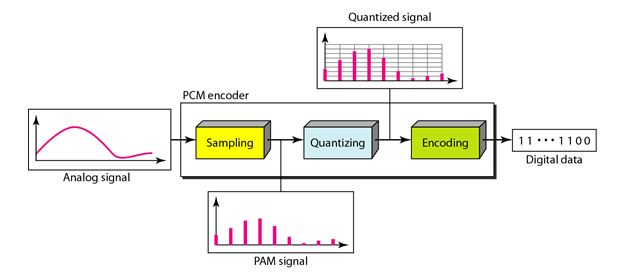
Pulse Code Modulation (PCM) is the most common technique used to change an analog signal to digital data (digitization). A PCM encoder has three processes as shown in the following Figure.
The analog signal is sampled.
The sampled signal is quantized.
The quantized values are encoded as streams of bits.
Sampling
The first step in PCM is sampling. The analog signal is sampled every Ts s, where Ts is the sample interval or period. The inverse of the sampling interval is called the sampling rate or sampling frequency and denoted by ƒs, Where ƒs = 1/ Ts.
You May also Like:
Line Coding and Its Characteristics
Different Line Coding Techniques
Different Block Coding Techniques
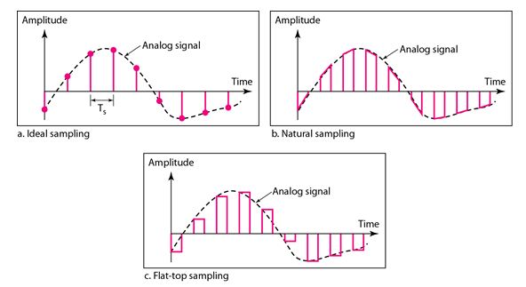
There are three sampling methods-ideal, natural, and flat-top. In ideal sampling, pulses from the analog signal are sampled. This is an ideal sampling method and cannot be easily implemented. In natural sampling, a high-speed switch is turned on for only the small period of time when the sampling occurs.
The result is a sequence of samples that retains the shape of the analog signal. The most common sampling method, called sample and hold, however, creates flat-top samples by using a circuit. The sampling process is sometimes referred to as pulse amplitude modulation (PAM). The different sampling methods are as shown in the following figure.
Sampling Rate
One important consideration is the sampling rate or frequency. What are the restrictions on Ts? According to the Nyquist theorem, to reproduce the original analog signal, one necessary condition is that the sampling rate be at least twice the highest frequency in the original signal.
As for this Theorem, First, we can sample a signal only if the signal is band-limited i.e a signal with an infinite bandwidth cannot be sampled. Second, the sampling rate must be at least 2 times the highest frequency, not the bandwidth. If the analog signal is low-pass, the bandwidth and the highest frequency are the same value. If the analog signal is bandpass, the bandwidth value is lower than the value of the maximum frequency.
Quantization
The result of sampling is a series of pulses with amplitude values between the maximum and minimum amplitudes of the signal. The set of amplitudes can be infinite with non-integral values between the two limits. These values cannot be used in the encoding process. The following are the steps in quantization:
1. We assume that the original analog signal has instantaneous amplitudes between Vmin and Vmax
2. We divide the range into L zones, each of height ∆ (delta).
∆=(Vmax-Vmin)/L
3. We assign quantized values of 0 to L - I to the midpoint of each zone.
4. We approximate the value of the sample amplitude to the quantized values.
As a simple example
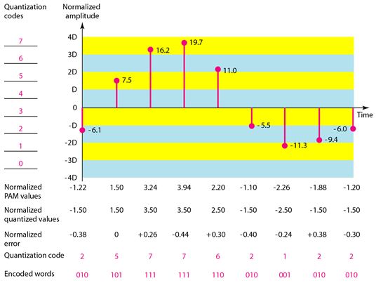
assume that we have a sampled signal and the sample amplitudes are between -20 and +20 V.
We decide to have eight levels (L = 8). This means that ∆ =5 V.
We have shown only nine samples using ideal sampling (for simplicity). The value at the top of each sample in the graph shows the actual amplitude. In the chart, the first row is the normalized value for each sample (actual amplitude/∆).
The quantization process selects the quantization value from the middle of each zone. This means that the normalized quantized values (second row) are different from the normalized amplitudes. The difference is called the normalized error (third row). The fourth row is the quantization code for each sample based on the quantization levels at the left of the graph. The encoded words (fifth row) are the final products of the conversion.
Quantization Levels:
In the above example, we showed eight quantization levels. The choice of L, the number of levels, depends on the range of the amplitudes of the analog signal and how accurately we need to recover the signal. If the amplitude of a signal fluctuates between two values only, we need only two levels; if the signal, like voice, has many amplitude values, we need more quantization levels. In audio digitizing, L is normally chosen to be 256; in video it is normally thousands. Choosing lower values of L increases the quantization error if there is a lot of fluctuation in the signal.
Quantization Error:
One important issue is the error created in the quantization process. Quantization is an approximation process. The input values to the quantizer are the real values; the output values are the approximated values. The output values are chosen to be the middle value in the zone. If the input value is also at the middle of the zone, there is no quantization error; otherwise, there is an error. In the previous example, the normalized amplitude of the third sample is 3.24, but the normalized quantized value is 3.50. This means that there is an error of +0.26. The value of the error for any sample is less than ∆/2. In other words, we have ∆/2<=error<= ∆/2.
Uniform Versus Non uniform Quantization:
For many applications, the distribution of the instantaneous amplitudes in the analog signal is not uniform. Changes in amplitude often occur more frequently in the lower amplitudes than in the higher ones. For these types of applications it is better to use nonuniform zones. In other words, the height of ∆ is not fixed; it is greater near the lower amplitudes and less near the higher amplitudes.
Nonuniform quantization can also be achieved by using a process called companding and expanding. The signal is companded at the sender before conversion; it is expanded at the receiver after conversion. Companding means reducing the instantaneous voltage amplitude for large values; expanding is the opposite process. Companding gives greater weight to strong signals and less weight to weak ones. It has been proved that nonuniform quantization effectively reduces the SNRdB of quantization.
Encoding
The last step in PCM is encoding. After each sample is quantized and the number of bits per sample is decided, each sample can be changed to an nb-bit code word. In the above figure the encoded words are shown in the last row. A quantization code of 2 is encoded as 010; 5 is encoded as 101; and so on. Note that the number of bits for each sample is determined from the number of quantization levels. If the number of quantization levels is L, the number of bits is nb=log2 L. In our example L is 8 and nb is therefore 3. The bit rate can be found from the formula.
Bitrate = Sampling rate X Number of bites per sample= ƒs X nb
II. Delta Modulation (DM)
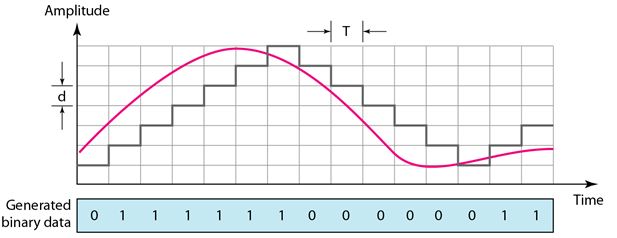
PCM is a very complex technique. Number of other techniques has been developed to reduce the complexity of PCM. The simplest is delta modulation. PCM finds the value of the signal amplitude for each sample; DM finds the change from the previous sample. The following figure shows the process. Note that there are no code words here; bits are sent one after another.
Modulator
The modulator is used at the sender site to create a stream of bits from an analog signal. The process records the small positive or negative changes, called delta . If the delta is positive, the process records a 1; if it is negative, the process records a 0. However, the process needs a base against which the analog signal is compared. The modulator builds a second signal that resembles a staircase. Finding the change is then reduced to comparing the input signal with the gradually made staircase signal.
The modulator, at each sampling interval, compares the value of the analog signal with the last value of the staircase signal. If the amplitude of the analog signal is larger, the next bit in the digital data is 1; otherwise, it is O. The output of the comparator, however, also makes the staircase itself. If the next bit is I, the staircase maker moves the last point of the staircase signal up; it the next bit is 0, it moves it down. Note that we need a delay unit to hold the staircase function for a period between two comparisons.
Demodulator
The demodulator takes the digital data and, using the staircase maker and the delay unit, creates the analog signal. The created analog signal, however, needs to pass through a low-pass filter for smoothing.
Adaptive DM
A better performance can be achieved if the value of is not fixed. In adaptive delta modulation, the value of changes according to the amplitude of the analog signal.
Quantization Error
It is obvious that DM is not perfect. Quantization error is always introduced in the process. The quantization error of DM, however, is much less than that for PCM.
You May Also Like:
Different Scrambling Techniques
Different Transmission Modes
Back to DCN Questions and Answers